Loading and processing data
1. Data Load
MNIST Dataset Load
from torchvision import datasets, transforms
path2data = './data'
# train_data = datasets.MNIST(path2data, train=True, download=True)
Downloading http://yann.lecun.com/exdb/mnist/train-images-idx3-ubyte.gz to ./data/MNIST/raw/train-images-idx3-ubyte.gz


0it [00:00, ?it/s]


Extracting ./data/MNIST/raw/train-images-idx3-ubyte.gz to ./data/MNIST/raw
Downloading http://yann.lecun.com/exdb/mnist/train-labels-idx1-ubyte.gz to ./data/MNIST/raw/train-labels-idx1-ubyte.gz


0it [00:00, ?it/s]


Extracting ./data/MNIST/raw/train-labels-idx1-ubyte.gz to ./data/MNIST/raw
Downloading http://yann.lecun.com/exdb/mnist/t10k-images-idx3-ubyte.gz to ./data/MNIST/raw/t10k-images-idx3-ubyte.gz


0it [00:00, ?it/s]


Extracting ./data/MNIST/raw/t10k-images-idx3-ubyte.gz to ./data/MNIST/raw
Downloading http://yann.lecun.com/exdb/mnist/t10k-labels-idx1-ubyte.gz to ./data/MNIST/raw/t10k-labels-idx1-ubyte.gz


0it [00:00, ?it/s]


Extracting ./data/MNIST/raw/t10k-labels-idx1-ubyte.gz to ./data/MNIST/raw
Processing...
Done!


/Users/ohhyunkwon/.virtualenvs/torch_oh/lib/python3.6/site-packages/torchvision/datasets/mnist.py:480: UserWarning: The given NumPy array is not writeable, and PyTorch does not support non-writeable tensors. This means you can write to the underlying (supposedly non-writeable) NumPy array using the tensor. You may want to copy the array to protect its data or make it writeable before converting it to a tensor. This type of warning will be suppressed for the rest of this program. (Triggered internally at  ../torch/csrc/utils/tensor_numpy.cpp:141.)
  return torch.from_numpy(parsed.astype(m[2], copy=False)).view(*s)
train_data = datasets.MNIST(path2data, train=True, download=False)
train_data
Dataset MNIST
    Number of datapoints: 60000
    Root location: ./data
    Split: Train
x_train, y_train = train_data.data, train_data.targets
print(x_train.shape)
print(y_train.shape)
torch.Size([60000, 28, 28])
torch.Size([60000])
# val_data = datasets.MNIST(path2data, train=False, download=True)
val_data = datasets.MNIST(path2data, train=False, download=False)
val_data
Dataset MNIST
    Number of datapoints: 10000
    Root location: ./data
    Split: Test
x_val, y_val = val_data.data, val_data.targets
print(x_val.shape)
print(y_val.shape)
torch.Size([10000, 28, 28])
torch.Size([10000])
Add New Dimension to Tensors
# unsqueeze(): 특정 위치에 1인 차원 추가
print(x_train.shape, x_train.unsqueeze(1).shape)
torch.Size([60000, 28, 28]) torch.Size([60000, 1, 28, 28])
if len(x_train.shape) == 3:
    x_train = x_train.unsqueeze(1)
print(x_train.shape)

if len(x_val.shape) == 3:
    x_val = x_val.unsqueeze(1)
print(x_val.shape)
torch.Size([60000, 1, 28, 28])
torch.Size([10000, 1, 28, 28])
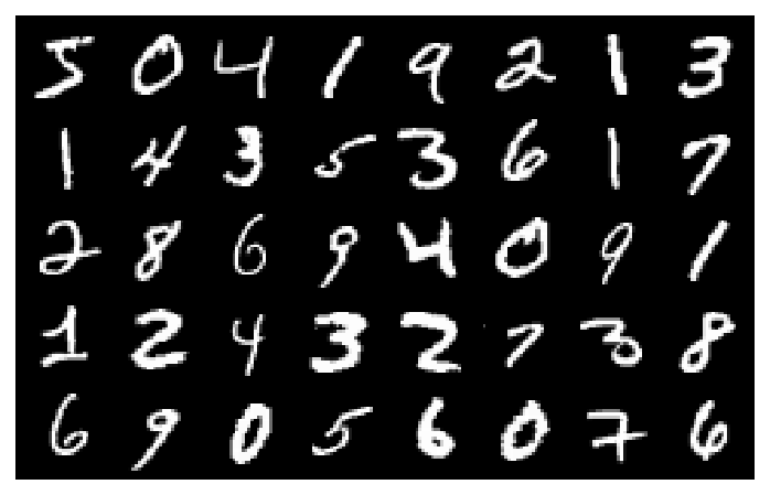
Display Sample Images
from torchvision import utils
import matplotlib.pyplot as plt
import numpy as np
# retina 옵션으로 해상도 올리기
from IPython.display import set_matplotlib_formats
set_matplotlib_formats('retina')
def show(img):
    # 텐서를 넘파이 array로 변환
    npimg = img.numpy()
    # H * W * C 모양으로 변환
    # np.transpose(대상, (바꾸고자하는 기존 차원 순서))
    npimg_tr = np.transpose(npimg, (1, 2, 0))
    plt.axis('off')
    plt.imshow(npimg_tr, interpolation='nearest')
# 40개의 이미지 격자 만들기 (한 행에 8개씩)
# padding 2로 각 숫자 사이 빈 공간 및 상하좌우 여백 조금씩 두게 함
x_grid = utils.make_grid(x_train[:40], nrow=8, padding=2)
print(x_grid.shape)
torch.Size([3, 152, 242])
show(x_grid)
2. Data Transformation
# torchvisison.Compose(): Composes several transforms together
data_transform = transforms.Compose([
    # torchvision.transforms.RandomHorizontalFlip(p=0.5): Horizontally flip the given image randomly with a given probability
    transforms.RandomHorizontalFlip(p=1),
    # torchvision.transforms.RandomVerticalFlip(p=0.5): Vertically flip the given image randomly with a given probability
    transforms.RandomVerticalFlip(p=1),
    # torchvision.transforms.ToTensor(): Convert a PIL Image or numpy.ndarray to tensor
    #
    transforms.ToTensor(),
])
data_transform
Compose(
    RandomHorizontalFlip(p=1)
    RandomVerticalFlip(p=1)
    ToTensor()
)
# get a sample image from training dataset
img = train_data[0][0]
img

# transform sample image
img_tr = data_transform(img)
# convert tensor to numpy array
img_tr_np = img_tr.numpy()
# show original and transformed images
plt.subplot(1, 2, 1)
plt.imshow(img, cmap='gray')
plt.title('original')
plt.subplot(1, 2, 2)
plt.imshow(img_tr_np[0], cmap='gray')
plt.title('transformed')
Text(0.5, 1.0, 'transformed')

MNIST 불러오면서 바로 transformations까지 같이 진행
# train_data = datasets.MNIST(path2data, train=True, download=True, transform=data_transform)
train_data = datasets.MNIST(path2data, train=True, download=False, transform=data_transform)
train_data
Dataset MNIST
    Number of datapoints: 60000
    Root location: ./data
    Split: Train
    StandardTransform
Transform: Compose(
               RandomHorizontalFlip(p=1)
               RandomVerticalFlip(p=1)
               ToTensor()
           )
3. Wrapping tensors into a dataset
from torch.utils.data import TensorDataset
# pytorch dataset 만들기
train_ds = TensorDataset(x_train, y_train)
val_ds = TensorDataset(x_val, y_val)
for x, y in train_ds:
    print(x.shape, y.item())
    break
torch.Size([1, 28, 28]) 5
4. Creating data loaders
DataLoader: Combines a dataset and a sampler, and provides an iterable over the given dataset.
The DataLoader supports both map-style and iterable-style datasets with single- or multi-process loading, customizing loading order and optional automatic batching (collation) and memory pinning.
# data loaders for training / validation datasets
from torch.utils.data import DataLoader
# create a data loader from dataset
train_dl = DataLoader(train_ds, batch_size=8)
val_dl = DataLoader(val_ds, batch_size=8)
# iterate over batches
for xb, yb in train_dl:
    print(xb.shape)
    print(yb.shape)
    break
torch.Size([8, 1, 28, 28])
torch.Size([8])
Building models
nn: collection of modules that provide common deep learning layers
- a module of layer of
nnreceives input tensors, computes output tensors, and holds the weights nn.Sequential,nn.Module
1. Defining a linear layer
import torch
from torch import nn
# input tensor dimension 64 * 1000
# torch.randn(size): Returns a tensor filled with random numbers from a normal distribution with mean 0 and variance 1 (also called the standard normal distribution)
input_tensor = torch.randn(64, 1000)
# linear layer with 1000 inputs and 100 outputs
# torch.nn.Linear(in_features, out_features, ...): Applies a linear transformation to the incoming data
linear_layer = nn.Linear(1000, 100)
# output of the linear layer
output = linear_layer(input_tensor)
print(output.size())
torch.Size([64, 100])
2. Defining models using nn.Sequential
nn.Sequential: A sequential container. Modules will be added to it in the order they are passed in the constructor.
from torch import nn
# define a two-layer model
# input layer nodes: 4, hidden layer nodes: 5, output layer nodes: 1
model = nn.Sequential(
    nn.Linear(4, 5),
    nn.ReLU(),
    nn.Linear(5, 1)
)
print(model)
Sequential(
  (0): Linear(in_features=4, out_features=5, bias=True)
  (1): ReLU()
  (2): Linear(in_features=5, out_features=1, bias=True)
)
3. Defining models using nn.Module
nn.Module: Base class for all neural network modules.
Your models should also subclass this class.
Modules can also contain other Modules, allowing to nest them in a tree structure. You can assign the submodules as regular attributes
- This method provides better flexibility for building customized models.
import torch.nn.functional as F
# implement bulk of the class
# model has two convolutional layers and two fully connected layers
class Net(nn.Module):
    def __init__(self):
        super(Net, self).__init__()

    def forward(self, x):
        pass
model = Net()
print(model)
Net()
torch.nn.Conv2d
torch.nn.Conv2d(in_channels, out_channels, kernel_size, stride=1, padding=0, dilation=1, groups=1, bias=True, padding_mode=’zeros’, device=None, dtype=None)
# define __init__, forward function
class Net(nn.Module):
    def __init__(self):
        super(Net, self).__init__()
        self.conv1 = nn.Conv2d(1, 20, 5, 1)
        self.conv2 = nn.Conv2d(20, 50, 5, 1)
        self.fc1 = nn.Linear(4 * 4 * 50, 500)
        self.fc2 = nn.Linear(500, 10)

    def forward(self, x):
        x = F.relu(self.conv1(x))
        x = F.max_pool2d(x, 2, 2)
        x = F.relu(self.conv2(x))
        x = F.max_pool2d(x, 2, 2)
        # Tensor.view(*shape) → Tensor: Returns a new tensor with the same data as the self tensor but of a different shape.
        x = x.view(-1, 4 * 4 * 50)
        x = F.relu(self.fc1(x))
        x = self.fc2(x)
        # torch.nn.functional.log_softmax(input, dim=None, ...): Applies a softmax followed by a logarithm.
        # dim(int): A dimension along which log_softmax will be computed.
        return F.log_softmax(x, dim=1)
model = Net()
print(model)
Net(
  (conv1): Conv2d(1, 20, kernel_size=(5, 5), stride=(1, 1))
  (conv2): Conv2d(20, 50, kernel_size=(5, 5), stride=(1, 1))
  (fc1): Linear(in_features=800, out_features=500, bias=True)
  (fc2): Linear(in_features=500, out_features=10, bias=True)
)
Moving the model to a CUDA device (local MAC does not support)
print(next(model.parameters()).device)
cpu
# device = torch.device("cuda:0")
# model.to(device)
# print(next(model.parameters()).device)
4. Printing the model summary
torchsummary: package to get a summary of the model to see the output shape and the number of parameters in each layer.
from torchsummary import summary
summary(model, input_size=(1, 28, 28))
----------------------------------------------------------------
        Layer (type)               Output Shape         Param #
================================================================
            Conv2d-1           [-1, 20, 24, 24]             520
            Conv2d-2             [-1, 50, 8, 8]          25,050
            Linear-3                  [-1, 500]         400,500
            Linear-4                   [-1, 10]           5,010
================================================================
Total params: 431,080
Trainable params: 431,080
Non-trainable params: 0
----------------------------------------------------------------
Input size (MB): 0.00
Forward/backward pass size (MB): 0.12
Params size (MB): 1.64
Estimated Total Size (MB): 1.76
----------------------------------------------------------------
Defining the loss function and optimizer
loss function: computes the distance between the model outputs and targets. (objective function, cost function, criterion)
- e.g. classification problems: cross-entropy loss
optimizer: updates the model parameters (also called weights) during training.
optim: provides implementations of various optimization alogrithms.- e.g. Stochastic Gradient Descent(SGD), Adam, RMSprop
1. Defining the loss function
# defining a loss function, testing it on a mini-batch
# nn.NLLLoss(): The negative log likelihood loss. It is useful to train a classification problem with C classes.
# If provided, the optional argument weight should be a 1D Tensor assigning weight to each of the classes.
# This is particularly useful when you have an unbalanced training set.
loss_func = nn.NLLLoss(reduction='sum')
# test the loss function on a mini-batch
for xb, yb in train_dl:
    # move batch to cuda device
    # xb = xb.type(torch.float).to(device)
    # yb = yb.to(device)

    # get model output
    xb = xb.type(torch.float)
    out = model(xb)

    # calculate loss value
    loss = loss_func(out, yb)
    print(loss.item())
    break
68.28255462646484
# compute gradients
loss.backward()
2. Defining the optimizer
from torch import optim
# iterable parameters
model.parameters()
<generator object Module.parameters at 0x7fda47b270f8>
for param in model.parameters():
    print(param.shape)
    break
torch.Size([20, 1, 5, 5])
# defining Adam optimizer
# torch.optim.Adam(params, ...)
# params(iterable): iterable of parameters to optimize or dicts defining parameter groups
opt = optim.Adam(model.parameters(), lr=1e-4)
opt
Adam (
Parameter Group 0
    amsgrad: False
    betas: (0.9, 0.999)
    eps: 1e-08
    lr: 0.0001
    weight_decay: 0
)
# update model parameters
# torch.optim.Adam.step: Performs a single optimization step.
opt.step()
# set gradients to zero
# torch.optim.Adam.zero_grad: Sets the gradients of all optimized 'torch.Tensor's to zero.
opt.zero_grad()
3. Training and evaluation
Develop a helper function to compute the loss value per mini-batch
def loss_batch(loss_func, xb, yb, yb_h, opt=None):
    # obtain loss
    loss = loss_func(yb_h, yb)

    # obtain performance metric
    metric_b = metrics_batch(yb, yb_h)

    if opt is not None:
        loss.backward()
        opt.step()
        opt.zero_grad()

    return loss.item(), metric_b
Define a helper function to compute the accuracy per mini-batch
def metrics_batch(target, output):
    # obtain output class
    # torch.argmax(input, dim, keepdim=False) → LongTensor
    # Returns the indices of the maximum values of a tensor across a dimension.
    # - input(Tensor): the input tensor.
    # - dim(int): the dimension to reduce. If None, the argmax of the flattened input is returned.
    # - keepdim(bool): whether the output tensor has dim retained or not. Ignored if dim=None.
    pred = output.argmax(dim=1, keepdim=True)

    # compare output class with target class

    # torch.eq(input, other, *, out=None) → Tensor
    # Computes element-wise equality
    # The second argument can be a number or a tensor whose shape is broadcastable with the first argument.
    # - input(Tensor): the tensor to compare
    # - other(Tensor or float): the tensor or value to compare

    # Tensor.view_as(other) → Tensor
    # View this tensor as the same size as other. self.view_as(other) is equivalent to self.view(other.size()).
    corrects = pred.eq(target.view_as(pred)).sum().item()

    return corrects
Define a helper function to compute the loss and metric values for a dataset
def loss_epoch(model, loss_func, dataset_dl, opt=None):
    loss = 0.0
    metric = 0.0
    len_data = len(dataset_dl.dataset)
    for xb, yb in dataset_dl:
        # xb = xb.type(torch.float).to(device)
        xb = xb.type(torch.float)
        # yb = yb.to(device)

        # obtain model output
        yb_h = model(xb)

        loss_b, metric_b = loss_batch(loss_func, xb, yb, yb_h, opt)
        loss += loss_b
        if metric_b is not None:
            metric += metric_b

    loss /= len_data
    metric /= len_data

    return loss, metric
Define the train_val function
def train_val(epochs, model, loss_func, opt, train_dl, val_dl):
    for epoch in range(epochs):
        # training mode
        model.train()
        train_loss, train_metric = loss_epoch(model, loss_func, train_dl, opt)

        # evaluation mode
        model.eval()
        # torch.no_grad()
        # Context-manager that disabled gradient calculation.
        # Disabling gradient calculation is useful for inference, when you are sure that you will not call Tensor.backward().
        # It will reduce memory consumption for computations that would otherwise have requires_grad=True.
        # In this mode, the result of every computation will have requires_grad=False, even when the inputs have requires_grad=True.
        # This context manager is thread local; it will not affect computation in other threads.
        # Also functions as a decorator. (Make sure to instantiate with parenthesis.)
        with torch.no_grad():
            val_loss, val_metric = loss_epoch(model, loss_func, val_dl)
        accuracy = 100 * val_metric

        print("epoch: %d, train loss: %.6f, val loss: %.6f, accuracy: %.2f" %(epoch, train_loss, val_loss, accuracy))
Train the model for a few epochs
model
Net(
  (conv1): Conv2d(1, 20, kernel_size=(5, 5), stride=(1, 1))
  (conv2): Conv2d(20, 50, kernel_size=(5, 5), stride=(1, 1))
  (fc1): Linear(in_features=800, out_features=500, bias=True)
  (fc2): Linear(in_features=500, out_features=10, bias=True)
)
loss_func
NLLLoss()
opt
Adam (
Parameter Group 0
    amsgrad: False
    betas: (0.9, 0.999)
    eps: 1e-08
    lr: 0.0001
    weight_decay: 0
)
train_dl
<torch.utils.data.dataloader.DataLoader at 0x7fda46553e10>
val_dl
<torch.utils.data.dataloader.DataLoader at 0x7fda46553dd8>
# call train_val function
num_epochs = 5
train_val(num_epochs, model, loss_func, opt, train_dl, val_dl)
epoch: 0, train loss: 0.148757, val loss: 0.065733, accuracy: 97.92
epoch: 1, train loss: 0.047690, val loss: 0.051643, accuracy: 98.35
epoch: 2, train loss: 0.026132, val loss: 0.052601, accuracy: 98.62
epoch: 3, train loss: 0.018569, val loss: 0.055401, accuracy: 98.66
epoch: 4, train loss: 0.014280, val loss: 0.052832, accuracy: 98.86
4. Storing and loading models
method 1
storing trained parameters in a file for deployment and future use
# define path2weights
path2weights = "./models/weights.pt"
# store state_dict to file
torch.save(model.state_dict(), path2weights)
loading the model parameters from the file
# define model: weights are randomly initiated
_model = Net()
# load state_dict from the file
weights = torch.load(path2weights)
# set state_dict to the model
_model.load_state_dict(weights)
<All keys matched successfully>
_model
Net(
  (conv1): Conv2d(1, 20, kernel_size=(5, 5), stride=(1, 1))
  (conv2): Conv2d(20, 50, kernel_size=(5, 5), stride=(1, 1))
  (fc1): Linear(in_features=800, out_features=500, bias=True)
  (fc2): Linear(in_features=500, out_features=10, bias=True)
)
method 2
# define path2model
path2model = "./models/model.pt"
# store model and weights into a file
torch.save(model, path2model)
# define model: weights are randomly initiated
_model = Net()
# load the model from the local file
_model = torch.load(path2model)
_model
Net(
  (conv1): Conv2d(1, 20, kernel_size=(5, 5), stride=(1, 1))
  (conv2): Conv2d(20, 50, kernel_size=(5, 5), stride=(1, 1))
  (fc1): Linear(in_features=800, out_features=500, bias=True)
  (fc2): Linear(in_features=500, out_features=10, bias=True)
)
5. Deploying the model
Once the model has been loaded into memory, we can pass new data to the model
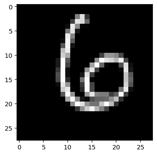
Sample tensor
# get a sample tensor
n = 100
x = x_val[n]
y = y_val[n]
print(x.shape)
plt.imshow(x.numpy()[0], cmap='gray')
torch.Size([1, 28, 28])


<matplotlib.image.AxesImage at 0x7fda47c98080>
Preprocess the tensor
# we use unsqueeze to expand dimensions to 1 * C * H * W
x = x.unsqueeze(0)
x.shape
torch.Size([1, 1, 28, 28])
# convert to torch.float32
x = x.type(torch.float)
x.type()
'torch.FloatTensor'
# move to cuda device
# x = x.to(device)
Get the model prediction
# get model output
output = _model(x)
output
tensor([[-36.4784, -35.5031, -40.6827, -41.9933, -28.2125, -22.9492,   0.0000,
         -46.7921, -31.0788, -45.1914]], grad_fn=<LogSoftmaxBackward>)
# get predicted class
pred = output.argmax(dim=1, keepdim=True)
pred
tensor([[6]])
print(pred.item(), y.item())
6 6